4.2. Neural Network Regularization

Regularization in Neural Networks

Regularization refers to methods that improve generalization by reducing a model’s effective capacity, variance, or sensitivity to noise. Unlike normalization layers, which stabilize optimization, regularizers shape the hypothesis space to avoid overfitting.

Regularization operates through different methods, including penalties on parameters and averaging hypotheses to reduce variance:

• Weight decay adds an L2 penalty to the loss, such that the loss and gradient descent update rule become
  $L^{\prime }(\theta )=L(\theta )+\lambda \Vert \theta {\Vert }_2^2⟺\theta \leftarrow \theta -\eta ({\nabla }_{\theta }L+2\lambda \theta ).$
  Weight decay shrinks weights toward zero, encouraging smoother, lower-norm solutions that reduce model complexity and avoid sharp minima.
  • Statistically, it corresponds to MAP estimation under a Gaussian prior, lowering the variance of the estimator and improving generalization.
  • Because models start with small weight values, stopping gradient descent early (i.e., when the validation error stops decreasing) implicitly acts as weight decay.
    ‎
• Dropout randomly disables activations during training. For activation $z_i$:
  $z_i^{\prime }=\{\begin{array}{ll}0& \text{with probability }p\\ \frac{z_i}{1-p}& \text{otherwise}.\end{array}$
  It increases generalization by forcing redundant representations and reduces effective model capacity. At inference, dropout uses the expected activation by averaging over all possible combinations of input neurons.
  ‎
• Residual (skip) connections add the input of a layer directly to its output in-between blocks, such that $y=x+F(x)$, where $F(x)$ is a learned transformation (e.g., a feedforward block or attention module). They stabilize optimization by improving gradient flow by reducing the frequency of vanishing/shattered gradients, allowing very deep networks to train effectively, and encouraging solutions that remain close to the identity mapping when needed.
  ‎
• Model averaging reduces variance by combining multiple hypotheses rather than relying on a single model. It includes ensembling strategies and explicit averaging of parameters.
  • Ensembling works by training multiple models and combining their predictions (usually by averaging). Ways to differentiate models are not specified, and the main goal is to reduce variance and improve generalization.
  • Bagging is an ensembling method that samples $K$ bootstrap datasets, trains one model per dataset and then averages the predictions. It is very useful for smaller/noisier datasets and decorrelates models via resampling.
  • Mixture-of-Experts (MoEs) route each input to a subset of expert networks, assigning learned gating weights $g_i(x)$ (usually sparse) to each expert, such that
    $f(x)={\sum }_{i=1}^M{g}_i(x)f_i(x).$
    MoEs regularize by activating only a few experts per input, creating structured sparsity and specialized submodels that reduce overfitting.

Examples

Vanishing Gradients & ResNets

The deeper a neural network grows, the more likely it will suffer from vanishing gradients because downstream layers (i.e., earlier layers) are the product of many backpropagated gradients–any of which may be close to zero. This example explores one approach to address vanishing gradients.

For one, the vanishing gradient problem can arise from saturating activation functions, such as the sigmoid.

What’s the maximum gradient of the sigmoid function? $\sigma (x)=\frac{1}{1+e^{-x}}.$ Taking its derivative, we obtain ${\sigma }^{\prime }(x)=\frac{e^{-x}}{(1+e^{-x}{)}^2}=\sigma (x)(1-\sigma (x)).$ Since $\sigma \in (0,1)$, the maximum gradient ${\sigma }^{\prime }(x)=0.25$ occurs at $x=0.5$.

The sigmoid function is expressed as

Why might ReLU be more preferable than the sigmoid function in deep networks? $\text{ReLU}(x)=\max (0,x).$ Its gradient is simply ${\text{ReLU}}^{\prime }(x)=\{\begin{array}{ll}0& x<0\\ 1& x>0.\end{array}$ As such, the gradient takes its maximum value of 1 whenever x>0. In deeper networks, repeatedly multiplying gradients smaller than one can cause vanishing gradients, whereas ReLU preserves gradient magnitude in its active region. Note, however, that the dying ReLU problem can occur when neurons output zero for all inputs, causing their gradients to remain zero and preventing further learning.

The ReLU activation is expressed as

One common way to tackle vanishing gradients is by adding residual connections. The figure
below shows a simplified example of a residual block. Assume that the weights consist of an
affine layer with zero biases.

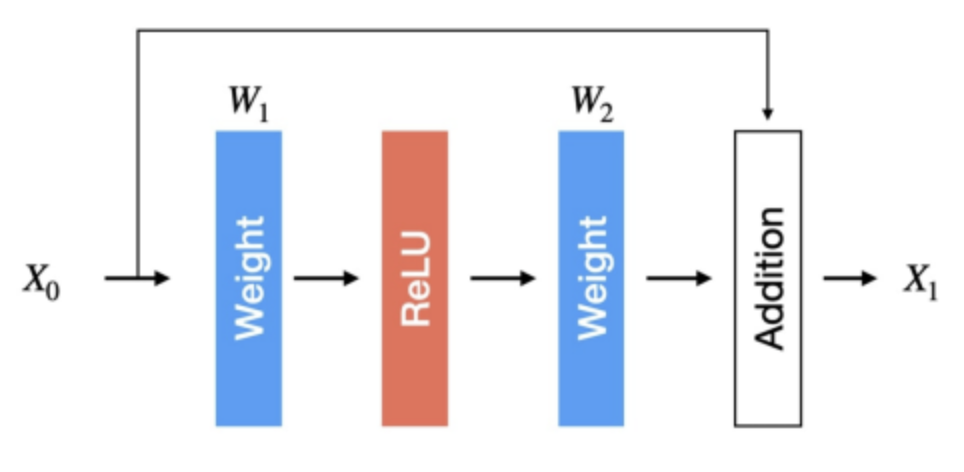
Write an expression for $X_1$ in terms of $W_1$, $W_2$ and $X_0$. We have two linear layers with a ReLU in between them. As such, $X_1=W_2\cdot \text{ReLU}(W_1{X}_0)+X_0.$

Assuming scalar variables, compute the gradient $\frac{\delta X_1}{\delta X_0}$. Based on what you see numerically, why does a residual connection preserve gradient norms better? We have that ${\Delta }_{X_0}{X}_1=W_2\cdot W_1\cdot {\text{ReLU}}^{\prime }(X_0)+1=\{\begin{array}{ll}1& X_0<0\\ W_1{W}_2+1& X_0>0.\end{array}$ When $X_0<0$, the ReLU unit is inactive and its gradient is zero, meaning the neuron itself is still “dead.” However, due to the additive skip connection, the total gradient remains equal to $1$, allowing gradients to propagate backward through the identity path. Thus, residual connections mitigate the effects of dying ReLU by preserving gradient flow, even though the ReLU unit itself remains inactive.

Dropout

In this example we explore dropout as a form of regularization.

Example