2.5b C-T Internal Stability

Stability in Continuous-Time LTI Difference Equation Model w/ No Input

For an input-less continuous-time LTI model $\frac{d}{dt}\vec{x}(t)=A\vec{x}(t)$ with $\vec{x}(0)={\vec{x}}_0$, where $A\in {\mathbb{R}}^{n\times n}$ has eigenvalues ${\lambda }_1,...,{\lambda }_n$, the model is:

1. Internally stable, if $\Re \{{\lambda }_i\}<0$ for all $i$.
2. Marginally stable, if

• $\Re \{{\lambda }_i\}\le 0$
• There exists at least one ${\lambda }_m$ where $\Re \{{\lambda }_m\}=0$
• All poles with a zero real part must be unique.

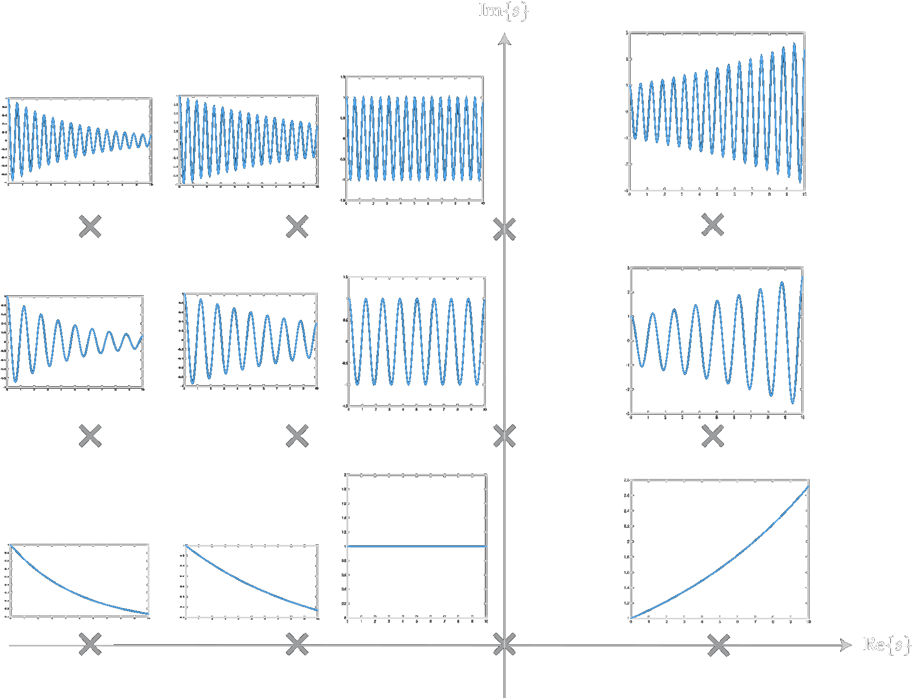
Continuous-time stability can be illustrated on the Cartesian plane as

\usepackage{tikz}
\usepackage{pgfplots}
\begin{document}
\begin{tikzpicture}
  % draw the coordinates
  \draw[->] (-2.5, 0) -- (2.5, 0) node[right] {$Re\{\lambda\}$};
  \draw[->] (0,-2.5) -- (0,2.5) node[above] {$Im\{\lambda\}$};
  \draw[->, thick, color=yellow] (0,-2.5) -- (0,2.5);
  \pgfsetfillopacity{0.25}
  % draw the unit circle
  \draw[thick, color=red!0, fill=red!30] (0,2.5)--(-2.5, 2.5)--(-2.5,-2.5)--(0,-2.5);
\end{tikzpicture}
\end{document}

Where the light-red-filled area ($Re\{\lambda \}<1$) is where internal stability is guaranteed, and the yellow line ($Re\{\lambda \}=1$) is where marginal stability may occur. Non-colored areas ($Re\{\lambda \}>0$) indicate where internal stability is guaranteed not to occur.

Intuition

Let’s first try to see why internal stability only happens in the above scenarios. Consider the input-less $\frac{d}{dx}{\vec{x}}_c(t)=A_c{\vec{x}}_c(t)$. The solution for this